Chapter 1 Accesing spatial data
In addition to the functions for statistical calculation that we have already seen, in R we can find several packages that allow to interact with spatial data, both in vector and raster format. Some of the main GIS packages in R are:
- rgdal
- Maptools
- raster
- GISTools
- Sp
Basically, these are libraries (packages) allow as reading and managing spatial data objects, such as ESRI shapefiles or raster files in ASCII format or any other GDAL supported format. These packages also allow you to create thematic maps from spatial data or to perform most of the geoprocesses of a Geographic Information System (GIS).
For the moment we will focus on packages raster and rgdal. We will see how to include some of their functions to automate some data extraction tasks. Specifically we will look at some examples of how to include these packages in regression models.
1.1 Working with vector layers
The Maptools package will allow us, among other things, to access information contained in spatial vector layers (points, lines and polygons). This package incorporates many other functions, but for the moment we will focus on the creation / import of space objects in R.
Vector information is characterized by representing elements by points, lines and polygons. Each of these elements is related to a record within an attribute table associated with spatial information. If you are not familiar with GIS or spatial data take a quick look to http://gisgeography.com/spatial-data-types-vector-raster/.
The Maptools package will allow us to import shapefiles1 and store them in spatial R objects such as:
- SpatialPointDataframe
- SpatialLineDataframe
- SpatialPolygonDataframe
In this way we can access both the spatial information (location) and thematic (attribute table). Let’s see an example using the stations.shp layer that you will find in the “shapes” folder on the course platform. This layer corresponds to the spatial location of part of the meteorological stations from which the information was obtained for the development of the linear regression practice.
You can download the script (vectorial.R) from the course platform with the instructions used.
1.1.1 Reading vector files
We will begin with installing and loading the packages:
install.packages('rgdal')
install.packages('maptools')
library(rgdal)
library(maptools)
We find several alternatives in the maptools package to access spatial vector information. Some of them are specific for each type of vector geometry (points, lines or polygons). There is, however, a generic function that operates on any geometry. This is the readOGR() function.
wStation<-readOGR('Data/weather_stations.shp') ## OGR data source with driver: ESRI Shapefile
## Source: "C:\Users\rmarc\Desktop\Copia_pen\European_Forestry_Master\module-3\Data\weather_stations.shp", layer: "weather_stations"
## with 95 features
## It has 10 fieldsWhen using this function we create an object of type SpatialDataframe. In this case, since the weather_stations.shp layer is a points layer, the wStation object is of type SpatialPointsDataframe. Spatial objects store all kinds of information related to spatial position (reference systems, extension …) and thematic features or attributes of objects.
To access the different parts of a spatialDataframe we will use the object name, the @ operator followed by the identifier of the section inside the object structure2. Thus, if we wanted to access the coordinates (Table 1.1) of the object station we would proceed as follows:
wStation@coordsFigure 1.1: Structure of the regression.txt file.
This coordinates are used to infer the real spatial location of echa point. An example of this may be calling the plot() function over wStation and observer the resulting plot:
plot(wStation)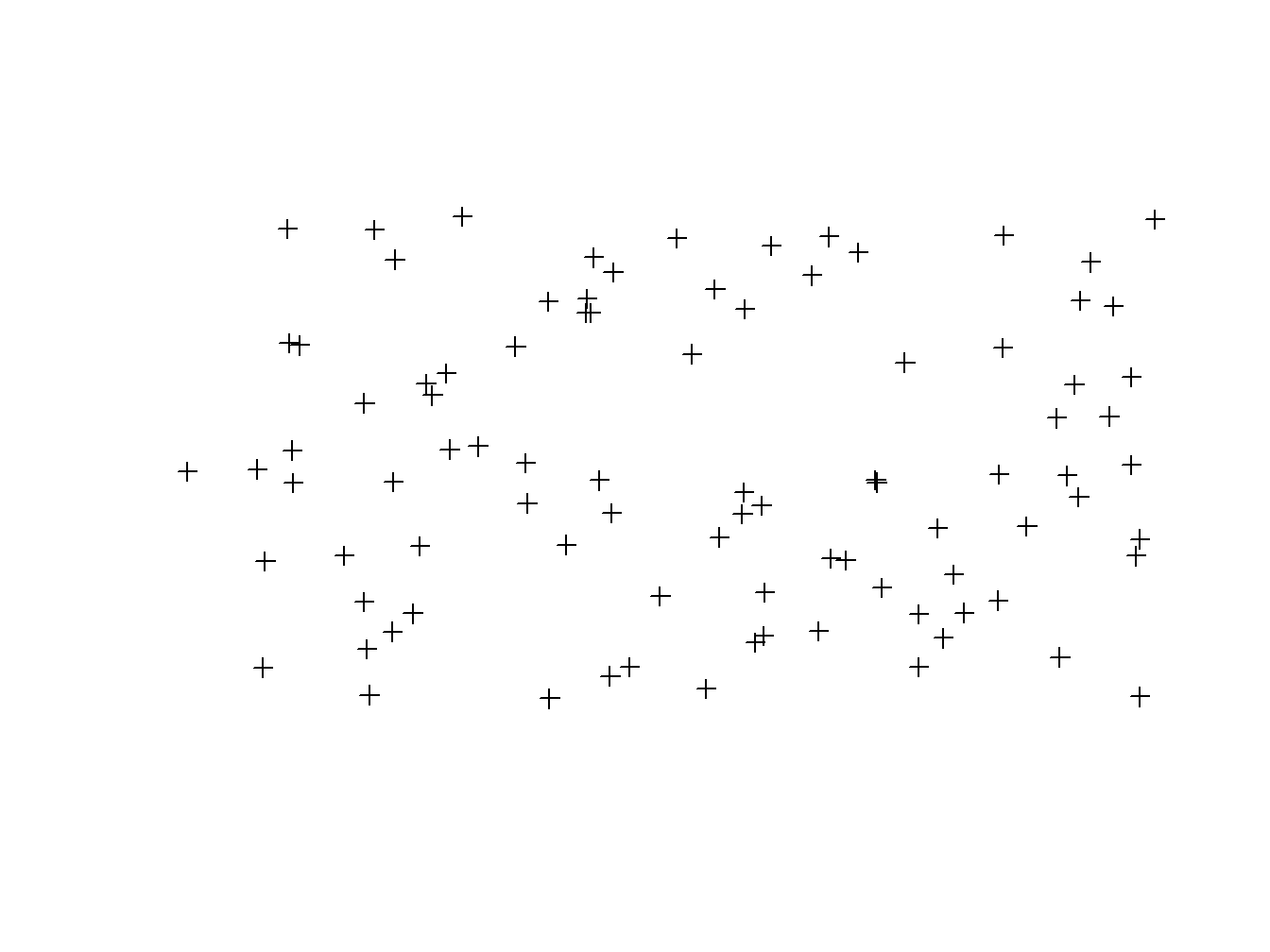
Take into account this is a regular dot plot so we can use other arguments:
plot(wStation, pch = 21, col='black', bg= 'red')
pointLabel(coordinates(wStation),labels=wStation$INDICATIVO,cex = 0.7)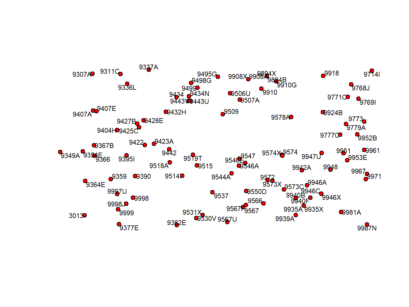
We are already familiar with some of them but the function `pointLabel()’ I new. In R there are thousands of functions and some of them are able to do the same. This one is just one of many choices we have to add labels to a spatial plot or map.
Finally, we can access the atribute table. In a vector layer, each feature (point in our case) is linked to a row of an atribute table. Both points and table are together in the SpatialPointsDataframe but we can access them separately. We have already seen how access coordinate information. To obtain the attribute table (Table 1.2)we do as follows:
wStation@dataFigure 1.2: Structure of the regression.txt file.
1.1.2 Querying and sampling vector layers
We have seen how to access the attributes of vector layers. This opens the door to a basic process in the field of spatial information processing, such as the selection of entities according to their attributes. At this point you will have already realized that the R philosophy is based on “recycling” functions. With this in mind, and knowing that the attribute table of a vector layer behaves in the same way as a data.frame does, you can get an idea of how the selection queries are implemented. In fact, it is done exactly the same as in the case of a normal data.frame. Let’s look at an example on the layer stations. We will select the points with an average temperature (Tmed_MES3) greater than 20:
wStation.Sel<- wStation[wStation$Tmed_MES>20,]
str(wStation.Sel@data)
## 'data.frame': 46 obs. of 10 variables:
## $ INDICATIVO: Factor w/ 95 levels "3013","9307A",..: 3 4 5 22 25 26 28 29 31 32 ...
## $ AÃ.O : num 2012 2012 2012 2012 2012 ...
## $ MES : num 6 6 6 6 6 6 6 6 6 6 ...
## $ NOMBRE : Factor w/ 94 levels "AGUARON P F E",..: 13 33 70 41 90 93 89 91 92 94 ...
## $ ALTITUD : num 440 455 228 370 247 198 221 258 262 225 ...
## $ T_MAX_abs : num 36.5 35 35 35 36.1 35.5 35.1 37.1 35 35.5 ...
## $ T_MIN_abs : num 9 11 10 9 10.4 11.9 12.4 11.9 10 9.7 ...
## $ TMed_MAX : num 26.8 26.7 27.9 27.1 28.2 28 27.9 28.4 25.8 27.5 ...
## $ TMed_MIN : num 14.6 14.7 15.1 14.6 15.6 15.9 16.4 15.9 14.8 13.6 ...
## $ Tmed_MES : num 20.7 20.7 21.5 20.9 21.9 ...So, according to the output from str() on wStation.Sel 46 points (or weather stations) recored an average temperature (in June) above 20\(C^\degree\). Now, since we have 2 spatial objects let’s try build a map to see the spatial location of our selected points:
plot(wStation, pch = 21, col='black', bg= 'red')
pointLabel(coordinates(wStation),labels=as.factor(wStation$Tmed_MES),cex = 0.7)
points(wStation.Sel, pch=21, col = 'yellow')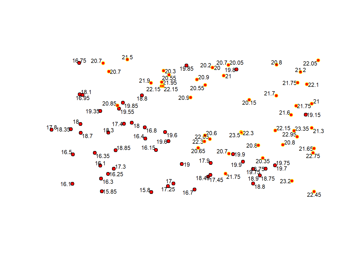
1.2 Working with raster layers
We have already seen how to access spatial information (GIS) in vector format using the maptools package. With this we could already read information from a layer in shapefile format and include it in a regression script as input data to create the dependent variable. In the next section we’ll do that.
The only thing we would have to do is to introduce the information related to the independent variables. For this we will use some of the functionalities available in the raster package. In this way we will also automate the obtaining of the independent variables.
The raster package provides utilities for manipulating geographic information in raster format. This package, along with maptools, converts R into a pseudo-GIS environment, allowing you to use most basic raster analysis functions. The raster package allows:
- Create raster objects.
- Manipulation of very heavy files.
- Map algebra and overlay functions.
- Distances and connection analysis.
- Conversion of polygons, lines and points to raster.
- Calculate spatial predictions of regression models.
- Mapping from raster maps.
- Reading and writing various types of raster files.
Of all these functionalities available we will focus on:
- Creating raster objects.
- Calculate predictions of regression models.
- Elaboration of maps.
- Reading and writing various types of raster files.
The remainnig functions can be found in a more intuitive way in any desktop GIS software. However, in some cases it may be more operative to use them directly in R.
The information in raster format is basically a 2-dimensional matrix, in which each of the grids or pixels is given a numerical value that represents either a category o parameter. This type of structure is particularly suitable to represent information about phenomena that has value in any location (continuous) such as elevation, temperature, distances… If we recall the independent variables used in the regression practice, they referred to phenomena of this nature. What we will do next is using the shapefile layer of weather stations to get information regarding the independent variables from raster layers.
1.2.1 Loading raster layers
Again, the most first thing to do is reading a raster layer. Once raster package is installed and loade we can call the raster() function and load any raster layer. Let’s see an example using the layer dem_rioja.tif that you can find in the folder Raster. It is a Digital Elevation Model (DEM)4 of the Autonomous Community of La Rioja5.
The first thing is to install the package. Unlike in other occasions this time we will specify the argument dep = TRUE. The raster package has many dependencies, ie, needs functions from other packages in order to work properly. It could be very annoying installing them one by one so we use that extra argument to ensure everything will work fine:
install.packages('raster', dep = TRUE)
library(raster)
Once installed and activated we can call the raster() function to read raster layer. Next we will use the plot() function to create a simple map of the raster layer we just read:
library(raster)
dem<-raster('Data/dem_rioja.tif')
plot(dem)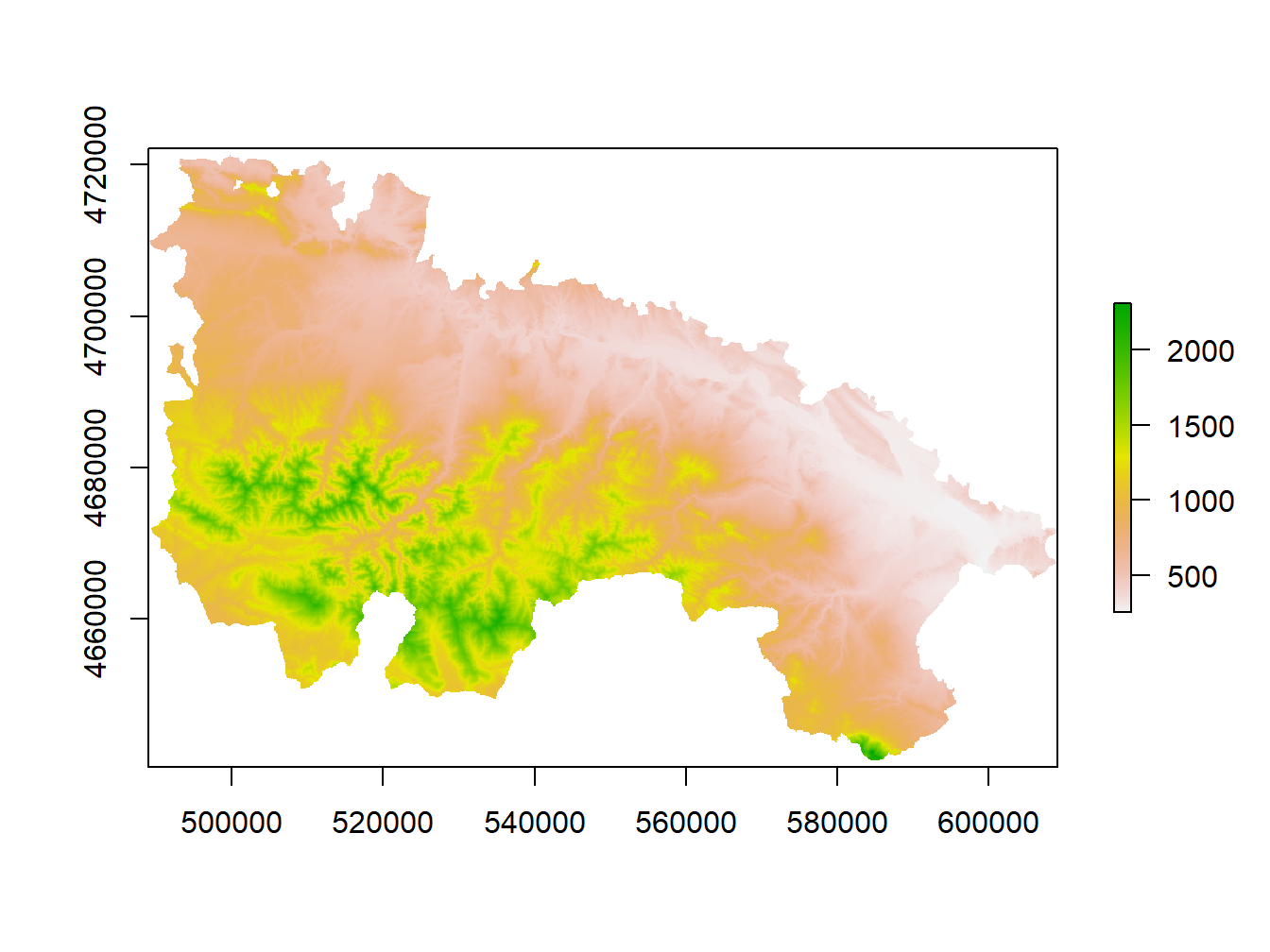
1.3 Loading multiple raster layers
Thanks to some of the utilities of the raster package we will be able to generate table-like objects with the values of multiple raster layers at once. We will use these data as input for our independent variables, but this is just an example. This procedure combines the location information of some input points (our weather stations) and raster layers with the information we want to retrieve. To do this we will use the stack() and extract() functions. ras The stack() function allows us to store several raster layers into a RasterStack array. Then we can interact with the RasterStack to extract information using the function extract(). The only thing we need to carry out this process is a list of coordinates that represent the locations from which we want to obtain the information. The most obvious example would be the location of the weather stations, for which we have already seen how to obtain in Working with vector layers. The process also involves using an specific fucntion to build a list with the location folder of the raster layers we want to load. Let’s begin with this last piece:
list.files('Data/variables_weather/',full.names = TRUE)## [1] "Data/variables_weather/d_atl.txt"
## [2] "Data/variables_weather/d_medit.txt"
## [3] "Data/variables_weather/lat.txt"
## [4] "Data/variables_weather/long.txt"
## [5] "Data/variables_weather/mde.txt"list.files is the most common approach in R to interact with our folder structure. It returns a vector with the names of the files in a given folder. In the first argument we pass a string with the location of the target folder. This is the only mandatory parameter, the remaing are optional. Among those optional we find:
full.names:TRUEorFALSEparameter that determines whether the function returns just file names or the complete path to each file. It is neededTRUEby `stack()’.pattern: paramater that allows filtering files by name.
Files containing txt:
list.files('Data/variables_weather/',full.names = TRUE, pattern = 'txt')## [1] "Data/variables_weather/d_atl.txt"
## [2] "Data/variables_weather/d_medit.txt"
## [3] "Data/variables_weather/lat.txt"
## [4] "Data/variables_weather/long.txt"
## [5] "Data/variables_weather/mde.txt"Files containing l:
list.files('Data/variables_weather/',full.names = TRUE, pattern = 'l')## [1] "Data/variables_weather/d_atl.txt"
## [2] "Data/variables_weather/lat.txt"
## [3] "Data/variables_weather/long.txt"Once we have our target list of files we can proceed with stack():
files<-list.files('Data/variables_weather/',full.names = TRUE, pattern = 'txt')
rasters<-stack(files)
Then we can manipulate it and inspect our new object:
head(rasters, n=10)## d_atl d_medit lat long mde
## [1,] 35106 336329 4758150 561250 NA
## [2,] 35117 336255 4758150 561350 NA
## [3,] 35128 336181 4758150 561450 NA
## [4,] 35140 336107 4758150 561550 NA
## [5,] 35151 336033 4758150 561650 NA
## [6,] 35163 335959 4758150 561750 NA
## [7,] 35176 335885 4758150 561850 NA
## [8,] 35188 335812 4758150 561950 NA
## [9,] 35201 335738 4758150 562050 NA
## [10,] 35215 335664 4758150 562150 NA
## [11,] 35205 336262 4758050 561250 NA
## [12,] 35216 336188 4758050 561350 492
## [13,] 35227 336114 4758050 561450 490
## [14,] 35239 336040 4758050 561550 473
## [15,] 35251 335966 4758050 561650 420
## [16,] 35263 335892 4758050 561750 389
## [17,] 35275 335818 4758050 561850 361
## [18,] 35288 335744 4758050 561950 396
## [19,] 35300 335670 4758050 562050 439
## [20,] 35314 335596 4758050 562150 458plot(rasters)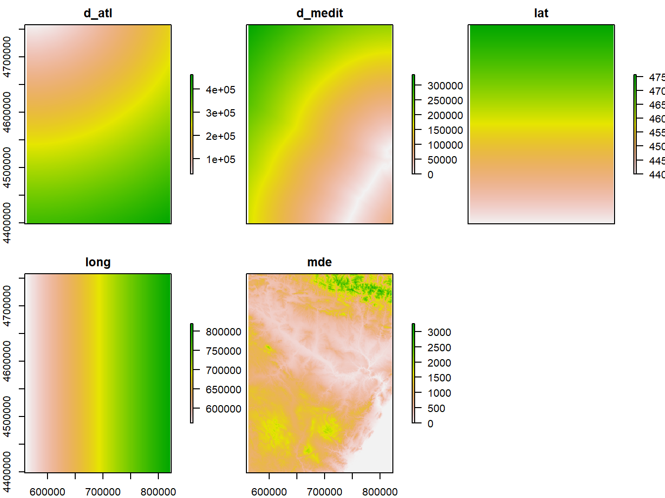
1.4 Spatial properties and characteristics
To end the basics of access to spatial layers let’s focus on seeing some fundamental properties that share all spatial layers. In essence we will see how to obtain and modify some parameters such as the extension of the layers or the reference system. In future modules we will go deeper into these concepts.
1.4.1 Layer extent
The layer extent is the rectangle that sorrounds spatial features, ie, the limits of data region. We can access the spatial extent of any layers with the extent() function. This function, which is common for both vector and raster layers, returns the coordinates of the ends of the layers:
extent(dem)## class : Extent
## xmin : 488974.8
## xmax : 609103.4
## ymin : 4641288
## ymax : 4721312extent(wStation)## class : Extent
## xmin : 574966
## xmax : 818327
## ymin : 4514365
## ymax : 4635648What good is this for us? Well, this can be used to know if our layers spatially match, to save this information and use it to cut layers or create empty raster “canvases” on which to dump information, for example the result of an interpolation process. In the short term, the greater utility of this function is to find out the units of the reference system in case we do not know the information.
1.4.2 Projections and reference system
The reference system (CRS) is a key element of spatial information. So far we have worked the spatial information without paying attention to this parameter. However, sooner or later we’ll have to deal with it. Not having taken this into account will give us problems. For example, we will not be able to overlay or combine layers by the absence or difference of reference systems, so we need to know how assing or reproject a layer to a different reference system.
1.4.2.1 Assign a Coordinate Reference System
A Coordinate Reference System or CRS must only be assign when a spatial layer lacks this information. Therefore, first we will see if our layers have or have not been assigned a reference system. A single function to do allows check and assing the CRS, crs(). We will apply this function on the layers wStations and dem:
crs(dem)## CRS arguments: NAcrs(wStation)## CRS arguments:
## +proj=tmerc +lat_0=0 +lon_0=30 +k=1 +x_0=500000 +y_0=0
## +ellps=intl +units=m +no_defsIn this particular case none of the layers were assigned a reference system. To give one first we have to know what system corresponds to them and how to assign it. The system that corresponds to them is the EPSG: 23030 - UTM ED50 30N. You can get a list of the different ways of coding reference systems at http://spatialreference.org/. In this case we will use the parameters according to the coding proj4 which is:
+proj=utm +zone=30 +ellps=intl +units=m +no_defsTo assign the CRS we proceed as follows:
crs(wStation)<-"+proj=utm +zone=30 +ellps=intl +units=m +no_defs"
crs(dem)<-"+proj=utm +zone=30 +ellps=intl +units=m +no_defs"
Finally, we check the CRS again:
crs(dem)## CRS arguments:
## +proj=utm +zone=30 +ellps=intl +units=m +no_defscrs(wStation)## CRS arguments:
## +proj=utm +zone=30 +ellps=intl +units=m +no_defs1.4.2.2 Layer projection
But, what if we want to change the CRS? Obviously in this case we can not use the above procedure. Furthermore, in this case, the same procedure is not used for each data model (vector or raster), but there is a function for the case of vector layers and another for raster layers. In the case of the vector layers we proceed as follows:
wStation.ETRS89<-spTransform(wStation,"+proj=utm +zone=30 +ellps=GRS80 +units=m +no_defs ")
crs(wStation.ETRS89)
## CRS arguments:
## +proj=utm +zone=30 +ellps=GRS80 +units=m +no_defsFor raster layes the procedure is similar but the funcion changes:
dem.ETRS89<-projectRaster(dem,crs=crs(wStation.ETRS89))
crs(dem.ETRS89)
## CRS arguments:
## +proj=utm +zone=30 +ellps=GRS80 +units=m +no_defsNote that in the raster example we retrieved the CRS from an existing layer rather than specify the CRS raw.
Something that is worth mention now is that we cannot project a layer that lacks CRS, first we have to assign it one.
There are other packages to do this like
rgeos.↩you can take a look at the structure using
str()as always, although you will see that this type of objects is much more complex than we have seen so far.↩Sorry, I know headers are in Spanish. We will rename them later I promise.↩
A DEM is a raster layer that takes elevation value in each pixel.↩
retrieved from http://centrodedescargas.cnig.es/CentroDescargas/index.jsp↩